Range Searching and Multi Dimensional Data

Intro

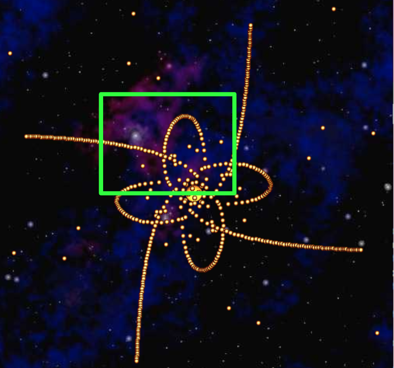
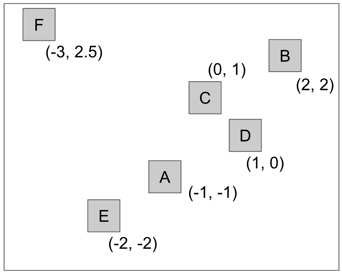
Let us consider a use case where we have a bunch of data points corresponding to X-Y coordinates of celestial bodies orbiting a sun, and we need to calculate the number of these bodies in a certain 2D range of coordinates, as shown below. Or we might need to find the closest body to a particular one.

These operations can be listed as follows:

• 2D range searching
• Nearest neighbors

.

If the data is stored as a hash table (the hashcode could be implemented using x and y coordinates), both operations will be Θ(N), since we would have to iterate over all items in the hash table. Let's simplify this problem by partitioning the 2D space into bins.

Uniform Partitioning

The idea is to leverage the fact that by knowing the X and Y position, we can know which bucket of the hash table a particular point will fall in.

Assuming the points are evenly spread out, this would reduce the number of points we would have to look up for both operations. However, runtimes for both will still be Θ(N).

Trees vs Hash Tables

Let's think about the nature of these two data structures for this particular problem. Search trees are all about order. As such, finding the minimum item in a BST is Θ(log(N)), whereas, it's Θ(N) in a hash table. We can make use of this ordered nature of search trees to improve the performance of the spatial operations we're dealing with.

Building Trees of Two Dimensional Data

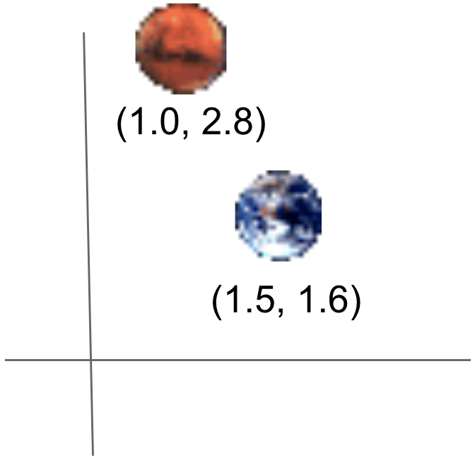
We need some way to compare these 2D points for storing them in a BST. These points have X and Y coordinates, and we could either one of them to compare points. But, we would have to choose either one of them, and stick with it. Let's consider an example of 2 2D points.

Based on whether we're using X or Y coordinates to compare, we'd end up with either one of the following BSTs.

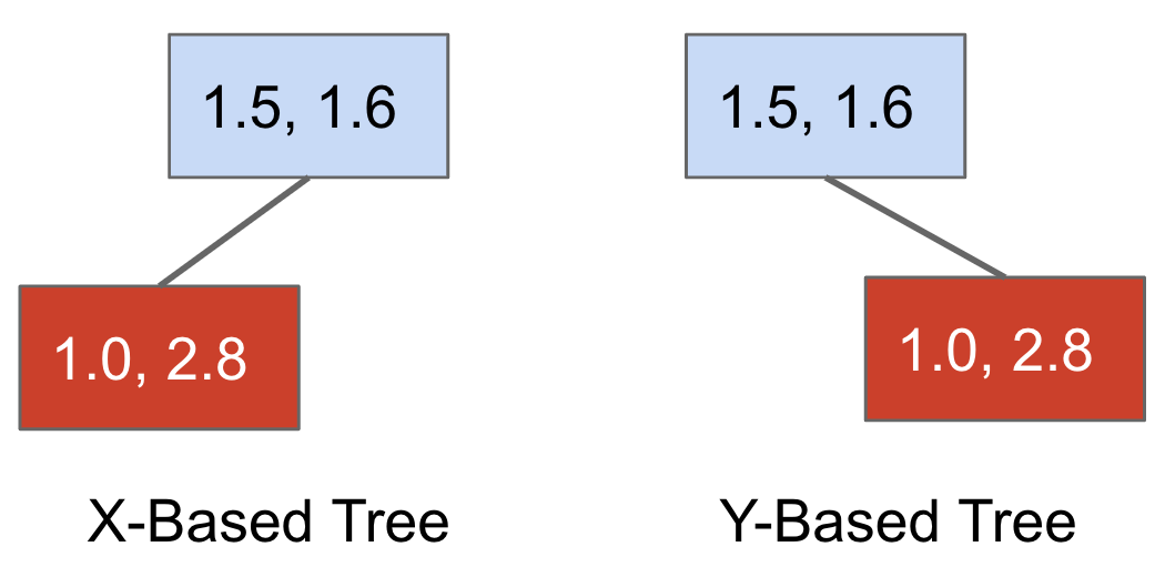
With both BST, we lose some representation of the spatial structure (since we're only using one dimension).

Let's see this in action. We'll see two trees representing a dataset of 6 2D points.

put((-1, -1), A)
put(( 2,  2), B)
put(( 0,  1), C)
put(( 1,  0), D)
put((-2, -2), E)
put((-3, 2.5), F)

Here's how they look in a 2D representation.

If we use the x-coordinate to compare, we get the following tree.

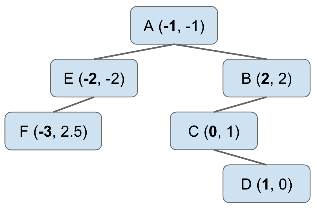
This is better than the original hash table based approach for certain operations. Suppose we want find out the points that have X coordinate less than -1.5. To do this we only need to look at the left hand child of the node A in the BST, and we can discard the right hand child completely. This process of cutting off tree search is called "pruning".

However, this won't work if we build the BST by comparing Y coordinates.

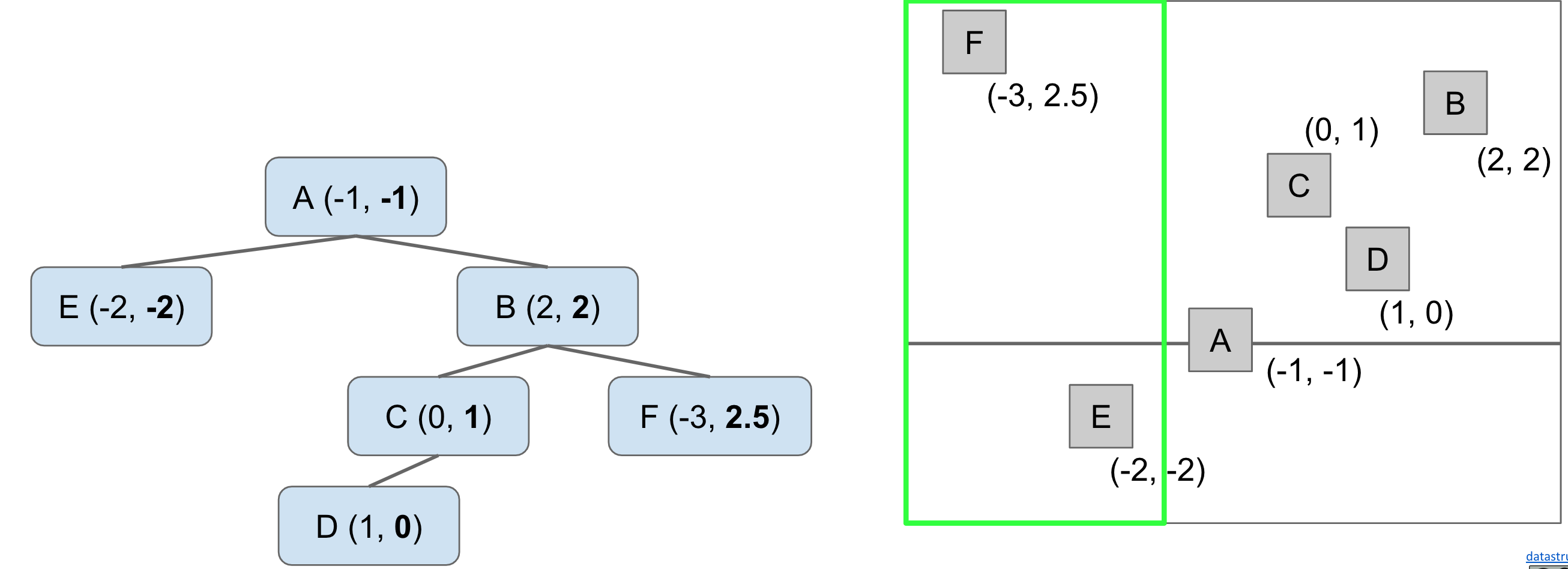
This shows the limitations of using just one coordinate to build the BST. Fortunately, we can do better than this.

QuadTree

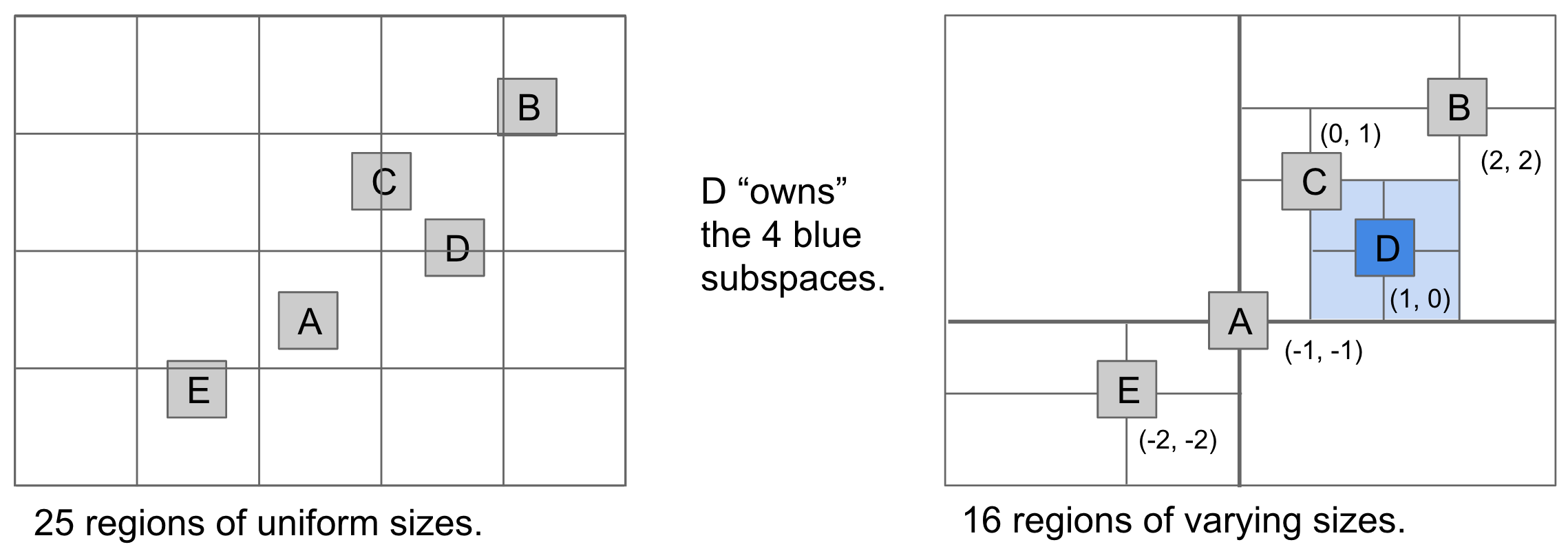
We can improve on the previous idea by building a search tree where every node has 4 neighbors, corresponding to northwest, northeast, southwest, and southeast directions.

As with regular BSTs, the order of insertion will determine the structure of the tree. Quadtrees are, in fact, spatial partitioning in disguise. The previous approach resulted in a uniform grid of rectangular regions, whereas we quadtrees we get what is called as hierarchical partitioning where each node "owns" 4 subspaces. Also, space is more finely divided in regions where there are more points.

Range Search

Let's see how the quadtree helps us out with the range search operation.

As seen in the video, the structure of the quadtree enabled us to prune links much more efficiently than the uniform partitioning approach.

KD Tree

k-d trees are an extension of the previous idea, one that handles arbitray number of dimensions. Let's see them in action using 2 dimensional data for the sake of simplicity.

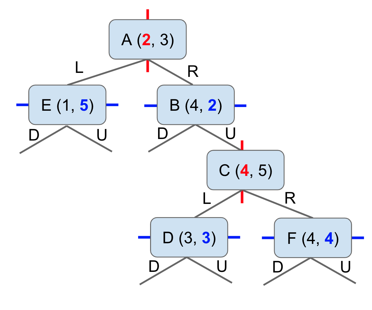
For the case of 2 dimensions, the basic idea is that the root partitions the entire space into left and right (ie, by the x dimension). All depth 1 nodes partition the subspace into up and down (ie, by the y dimension). We keep on cycling through the dimensions at each subsequent level.

Insertion

!!! note "We have to break ties somehow. We'll do that by saying that items that are equal in one dimension go off to the right child of each node."

Nearest Neighbor

Searching for a node in a k-d tree is similar to a quadtree, with the difference that each node in a k-d tree owns 2 subspaces instead of 4.

The intuition for finding the nearest neighbor using a k-d tree is that at any node, we want to look at the "good" side of its subtree before looking at the "bad" side.

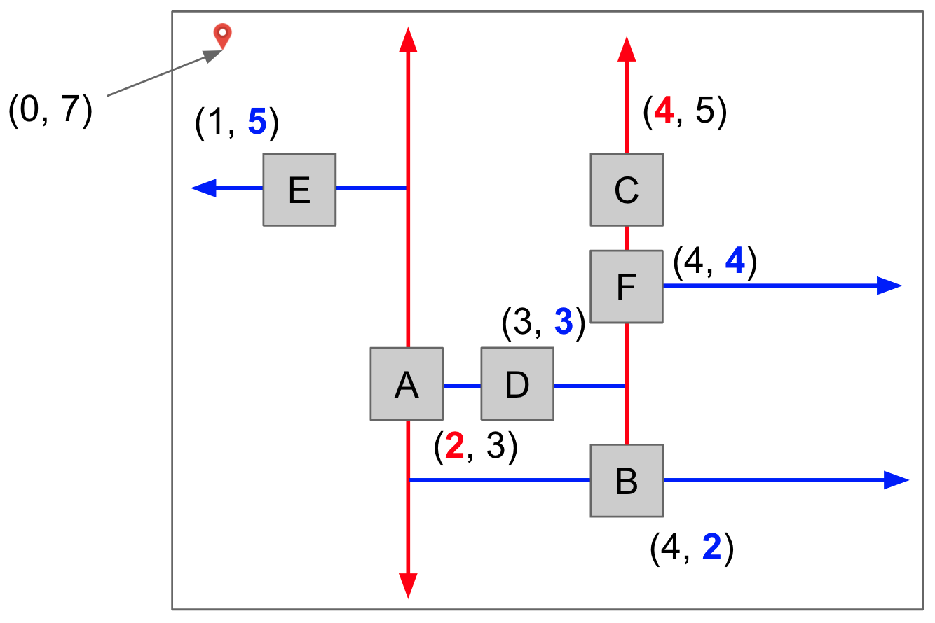
Let's understand that through a demo. Suppose we have the following k-d tree, and we need to find the node nearest to the point (0, 7).

The same tree in 2D representation is as follows.